Learn Pivot Tables: Excel Basics
You may use Excel to create and edit basic pivot table reports after reading this Blog. Learn about the characteristics of an Excel pivot table report, handle the limitations and compatibility difficulties associated with pivot tables, and determine when and why to utilize the Excel pivot table tool.
What is Pivot Tables ?
Excel's pivot table is an interactive tool. Typically, we enter raw information into Excel and want to obtain output according to requirements.
However, obtaining the intended result from raw data is challenging. Therefore, we must arrange the raw data. It can be difficult to correctly organize data in Excel. This complex task can be solved with a pivot table. We can arrange the data to suit our needs. Data can be readily arranged, created, and analyzed using a pivot table, which can then display the results according to requirements.
Life Before Pivot Tables!
Several formulas, such as SUM, COUNT, AVERAGE, IF, and VLOOKUP, had to be used before pivot tables.
Create separate summary tables by hand. Additionally, there is a high possibility of making a mistake.
2–3 hours to create summary report of 10,000 rows data.
Life after Pivot Tables!
Excel was transformed from a spreadsheet tool into a little data analysis engine by pivot tables.
Using a pivot table with 10,000 rows of data, it takes five to ten minutes.
Pivot tables provide professional reporting, speed, accuracy, and flexibility.
Comparison chart table:
| Before Pivot Table | After Pivot Table |
|---|---|
| Manual formulas | Drag & Drop |
| High error risk | Accurate aggregation |
| Time-consuming | Fast reporting |
| Static reports | Dynamic reports |
| Complex setup | User-friendly |
Why Should you use Excel pivot Tables?
pivot Table is the most important tool in Microsoft Excel toolset when yo look at your data set through it by your table you have the opportunity to see the details in the data that you might not have noticed.
Further more you can turn your data table to see your data from different perspectives.
With the help of pivot table firstly you can summarize large amount of data into meaningful information.
performing wide variety of calculation in a fraction of time
and you can quickly and easily categorize your data into groups.
How to Create pivot Table in Excel
You must place your arrow on the table in order for the pivot table tool to choose it automatically.
Simply click the insert button in the ribbon to create a pivot table, as seen in the image below with the black arrow.
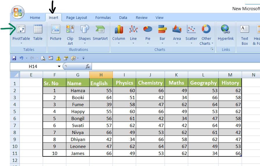
Next, choose the pivot table option, which is seen in the figure above with a green arrow.
As you can see in the figure below, clicking on pivot table opens the "Create pivotTable" dialog box.
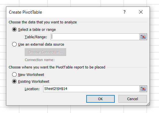
Next, choose the table in range. If you want to build a pivot table on a separate sheet, choose a new worksheet; if you want your pivot table on the same sheet, then choose the location.
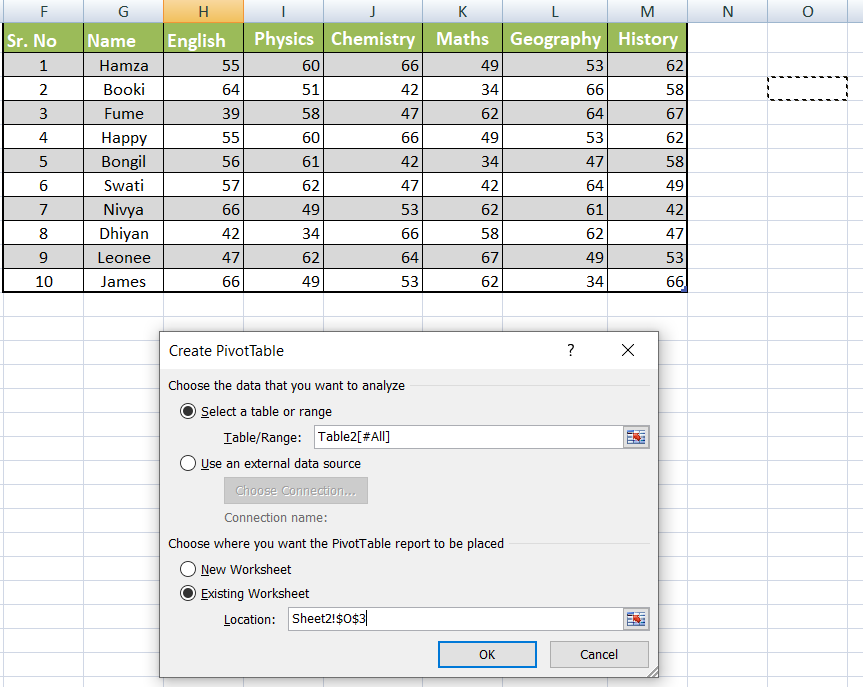
As you can see in the image below, I choose data in the table range and choose O3 column because I want my pivot table to be on the same sheet.
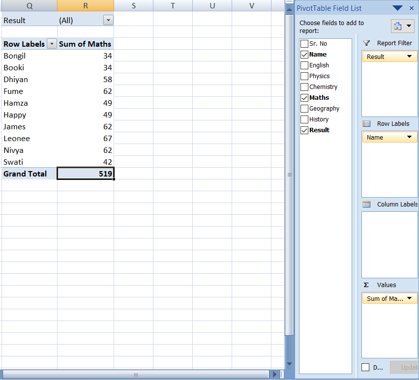
As you can see in the above image, I selected results as the report filter in the pick field. If you select topic, it appears in the row labels automatically, and if you select subject, it goes straight to values because we describe marks in all the subjects and you filter the table to see who is fail and who is pass, as shown in the image below.
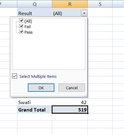
The student's name and grades are displayed if I use the fail filter.
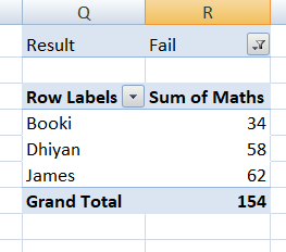
This is just an example of how you can simply separate your vast data with this table.