Top/Bottom Rules Explained Clearly
The conditional formatting features in Excel's Top and Bottom Rules let you quickly highlight the highest or lowest values in a range, making it easier to determine which values are highest or lowest.
A. Top 10 Item:
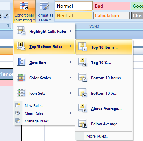
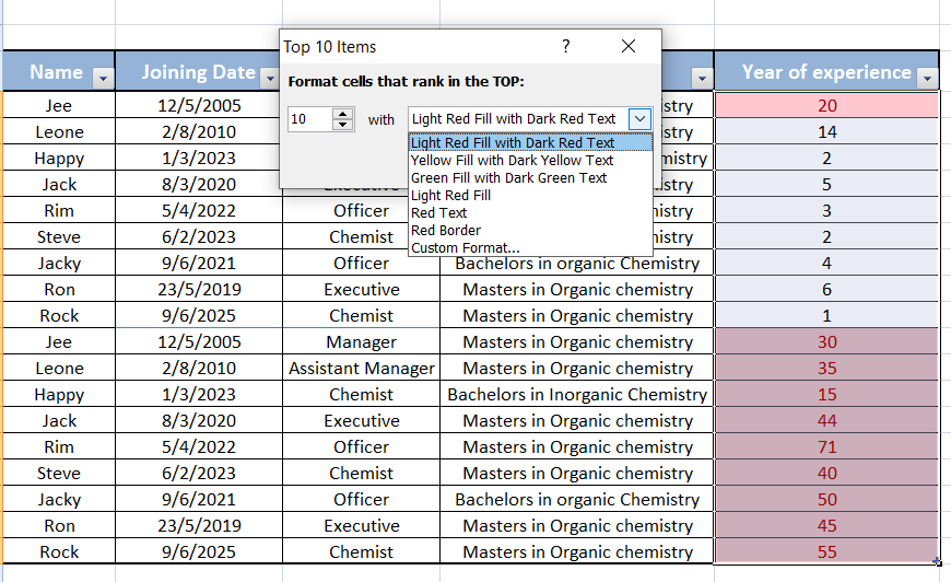
As you can see below, the greatest number more than 10 is indicated in red.
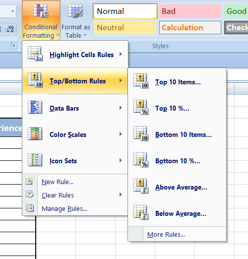
To format the top 10 items in Excel, you can follow these steps:
1. Select the range of cells containing the data you want to analyze.
2. Go to the "Home" tab on the Excel ribbon.
3. Click on the "Conditional Formatting" button in the Styles group.
4. Choose "Top/Bottom Rules" from the drop-down menu.
5. Select "Top 10 Items" from the sub-menu.
6. In the formatting dialog box that appears, you can select the formatting options you want to apply to the top 10 items.
7. Click "OK" to apply the formatting.
This will help you easily identify the top 10 items in your data set.
B. Top 10%:
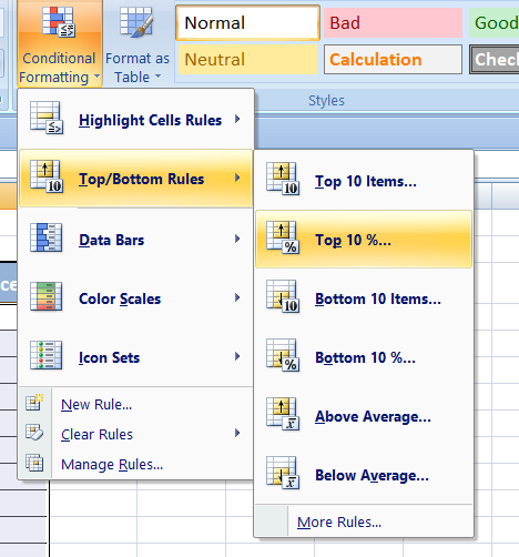
As you can see below, the greatest number more than 25% is indicated in Green.
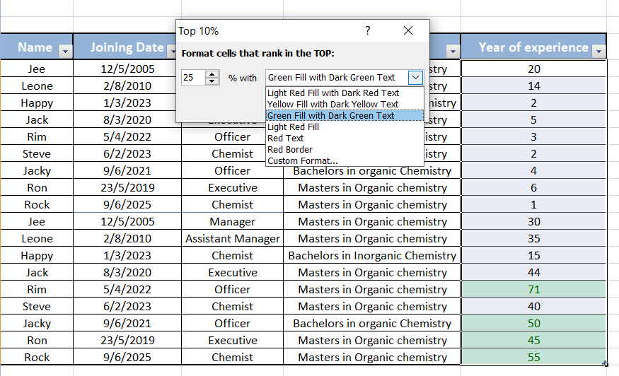
You may highlight the top 10% of values in a range of cells in Excel by using the Top 10% format in top/bottom rules, a conditional formatting option. It also means that the cells with the top 10% of values will have a different background color or be bolded, among other formatting changes. When you wish to rapidly determine which values in a dataset are the highest, this can be useful. The top 10% of values in a chosen range of cells are highlighted in Excel using the Top 10% format in top/bottom rules. A particular formatting style (such as a distinct font color, background color, or border) will be automatically applied by this formatting rule.
To apply this rule:
1. Select the range of cells you want to apply the formatting to.
2. Go to the Home tab on the Excel ribbon and click on the Conditional Formatting option.
3. Choose the Top/Bottom Rules option and then select Top 10% from the list of rule options.
4. In the dialog box that appears, you can customize the formatting options as needed, such as choosing the formatting style and color.
5. Click OK to apply the formatting rule to the selected range of cells.
C. Bottom 10 Items:
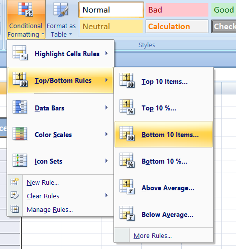
As you can see below, the greatest number less than 10 is indicated in Red.
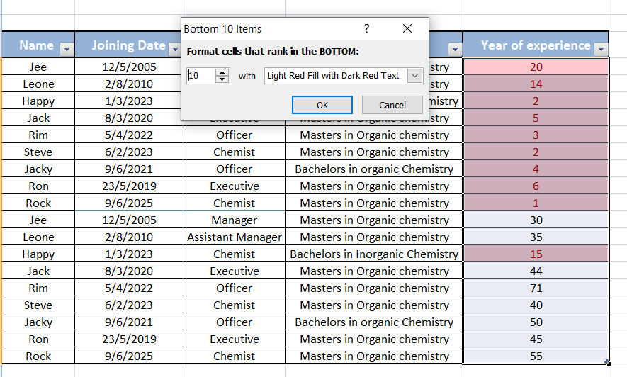
A conditional formatting rule that highlights the bottom 10 values in a chosen range of cells is Excel's "bottom 10 items" format in top/bottom rules. This can make it easier to find the number below 10. Choose the range of cells you wish to apply this formatting rule to, then in the Conditional Formatting menu, pick Top/Bottom Rules, and finally "Bottom 10 Items." After that, you can alter the formatting settings to what you prefer.
To apply the Bottom 10 items format rule in Excel, follow these steps:
1. Select the range of cells that you want to apply the formatting to.
2. Go to the "Home" tab on the Excel ribbon.
3. Click on the "Conditional Formatting" option in the Styles group.
4. Select "Top/Bottom Rules" from the drop-down menu.
5. Choose "Bottom 10 items" from the list of options.
6. Customize the formatting options as needed (such as changing the fill color, font color, etc.).
7. Click "OK" to apply the formatting rule.
D. Bottom 10%
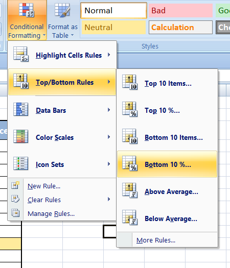
As you can see below, the greatest number less than 10% is indicated in yellow.
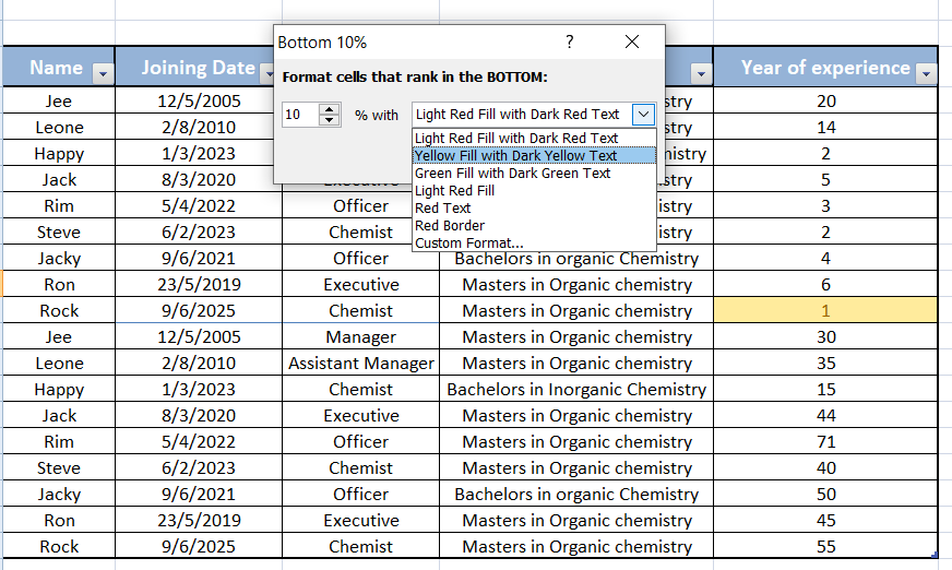
In Excel, the "Bottom 10%" format in top/bottom rules allows you to apply specific formatting (such as color, font style, etc.) to the lowest 10% of values in a range of cells. This can be useful for highlighting the lowest values in a data set or for visually distinguishing them from the rest of the values. The bottom 10% format in Excel refers to a conditional formatting rule that highlights the cells that fall within the lowest 10% of values in a selected range. This rule can be applied to a range of values to visually identify the lowest 10% of data points.
To apply the bottom 10% format in top/bottom rules in Excel, follow these steps:
1. Select the range of cells that you want to format.
2. Go to the "Home" tab on the Excel ribbon.
3. Click on the "Conditional Formatting" button in the Styles group.
4. Select "Top/Bottom Rules" from the drop-down menu.
5. Choose "Bottom 10%" from the options.
6. Customize the formatting options if desired.
7. Click "OK" to apply the formatting.
Once applied, the bottom 10% of values in the selected range will be highlighted with the specified formatting.
Click on below link to get further information-