Icon Sets in Excel for Dashboards

Icon Sets in Conditional Formatting in Excel are a way to visually categorize cell values using small icons (e.g., traffic lights, arrows, stars).

How to apply:

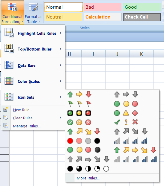
Go to Home > Conditional Formatting > Icon Sets.

Excel assigns icons based on the cell values relative to thresholds you choose (e.g., top 33% gets green, middle 33% yellow, bottom 34% red).

Rules can be based on, Percent of values, Number thresholds

You can customize the rule: reverse order, show only the icon (instead of the value), or set your own thresholds.

Works with numerical data (and can be used to compare across a range).

Example:

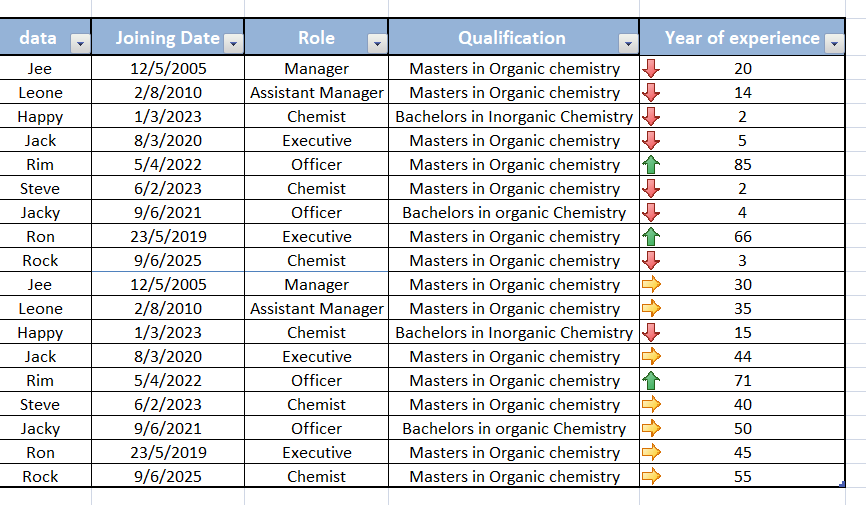
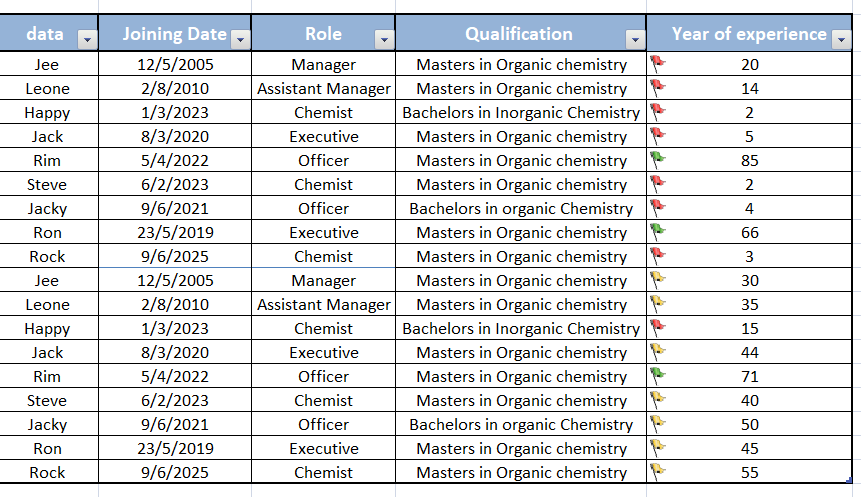
3-icon set (Green Arrow, Yellow Dash, Red X) Icon applied Sets to in sales Excel figures. Conditional Values Formatting above are 90th a percentile way show to green, add between small 50th icons and (like 90th arrows, show traffic yellow, lights, below stars) 50th to show cells red.

How to to visually adjust:

Classify After the applying, values, Helpful for quickly spotting high/low or good/bad performance.

How to use:

- Select the range.

- Home > Conditional Formatting > Icon Sets.

- Choose an icon style (e.g., 3 traffic lights, Icon 3 Sets arrows, are stars, a etc.).

- type Edit of the conditional rule formatting to in customize as below: